Menu
AI training failures can lead to poor performance, instability, or unsafe behavior in models. Common symptoms include low accuracy, erratic loss curves, or issues that emerge post-deployment. These failures are typically caused by problems in three areas: data quality, model design, and training setup. Addressing these issues early saves time, resources, and prevents business risks.
AI failures can harm business operations, delay launches, and increase costs. Debugging during training is far cheaper and more effective than fixing problems after deployment. Tools like TensorBoard, Optuna, or experiment tracking platforms can streamline the process, while external services like Artech Digital offer specialized support for complex issues.
The guide provides a step-by-step approach to identify and resolve common AI training problems, ensuring reliable and efficient model performance.
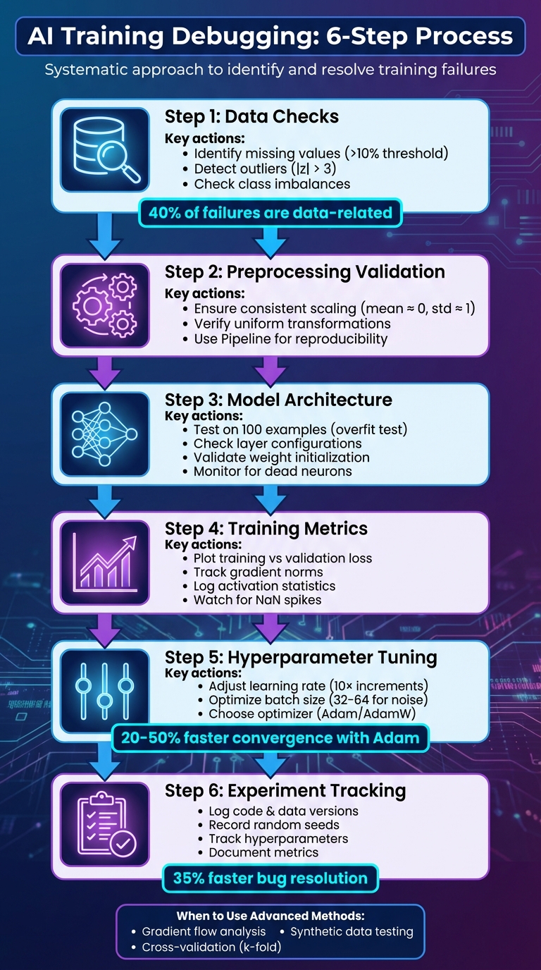
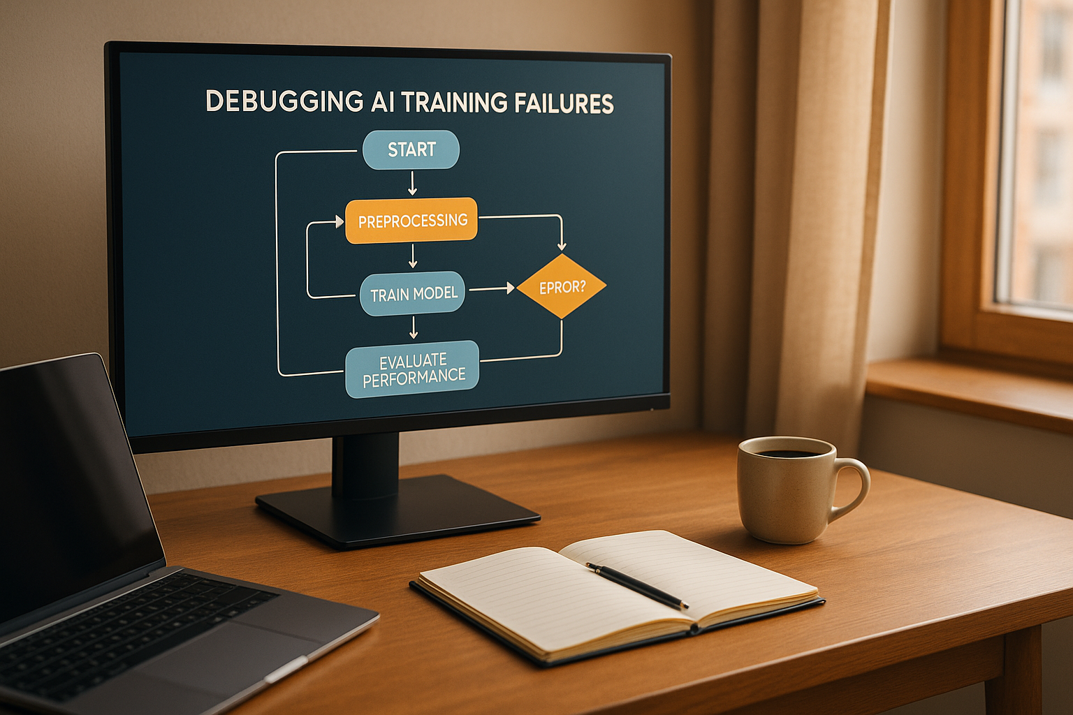
6-Step AI Training Debugging Process Flowchart
Data quality issues are a major cause of AI training failures - accounting for about 40%, according to analyses from Kaggle competitions. Before you even think about tweaking your model's architecture or adjusting hyperparameters, it's critical to ensure your dataset is in good shape. This means checking that it's clean, balanced, and formatted correctly. Common data issues include missing values, which leave gaps in your features, outliers, which can distort learning patterns, and imbalanced datasets, which may bias your model toward dominant classes. Let’s break down how to identify and address these problems.
The first step is to compute basic statistics to uncover potential issues. For missing values, a quick command like df.isnull().sum() in pandas will show how many values are missing for each feature. If you notice that a feature has 10% or more missing data, you can either fill in the gaps using the median - since it's less affected by outliers - or drop the feature entirely if it’s too sparse.
When it comes to outliers, methods like the z-score or interquartile range (IQR) are helpful. For the z-score, flag values where |z| > 3. Using the IQR approach, any value beyond 1.5× IQR is considered an outlier. Visual tools such as box plots can make spotting these anomalies easier. For example, in a housing price dataset, you might notice extreme values in the 99th percentile. To address this, you could clip prices above $1,000,000 to $950,000 to reduce their impact.
For imbalanced datasets, start by checking the class distribution with value_counts(). If you’re working with something like a fraud detection dataset and see a 100:1 ratio of legitimate to fraudulent transactions, your model might struggle to identify the minority class. Bar plots or pie charts can help visualize these imbalances. Research from Harvard’s robotics projects found that improving data variety and addressing sensor outliers boosted model performance by 20–30%.
| Issue Type | Detection Method | Fix Strategy |
|---|---|---|
| Missing Values | df.isnull().sum(), missingno.matrix() |
Impute (e.g., median/KNN) or drop feature |
| Outliers | Z-score ( | z |
| Class Imbalance | value_counts(), class ratio analysis |
Oversample (e.g., SMOTE) or adjust weights |
Once you’ve addressed these issues, it's time to verify that your preprocessing steps are consistent.
After cleaning your data, ensuring consistent preprocessing across datasets is crucial. Any mismatch between how training and validation sets are processed can lead to distribution shifts, which can skew your validation performance. For instance, if you standardize your data, make sure to fit the scaler only on the training set using scaler.fit(X_train) and then apply it to both training and validation sets with scaler.transform(). This ensures the mean and standard deviation are uniform - ideally, the mean should hover around 0, and the standard deviation should be close to 1.
To catch preprocessing errors early, use unit tests. For example, you can confirm consistent scaling with assertions like:
assert np.all((X_train_scaled - X_val_scaled).mean() < 1e-6)
For image data, verify that RGB channels are scaled consistently across all splits to avoid introducing unintended patterns. To streamline this process, consider using scikit-learn’s Pipeline class. This not only guarantees reproducibility but also minimizes the risk of manual mistakes. Keep in mind that preprocessing errors in deep learning workflows can sometimes go unnoticed until they cause unexpected performance drops. Packaging and testing your preprocessing steps can save you from such headaches down the line.
Once data issues are resolved, the next step is refining the model's architecture and training parameters. Common architecture problems can manifest in several ways: models that repeatedly output the same prediction, training loss that refuses to improve, or values that skyrocket to NaN within the first few batches. To tackle these issues, start by testing the model on a small, clean subset of data - about 100 examples - to see if it can overfit. If it fails to overfit, the problem likely lies in the model's configuration rather than the data or hyperparameters. This is your cue to take a closer look at the model's structure.
Start by thoroughly documenting your architecture, including details like layer types, input/output shapes, activations, and parameter counts. Run a dry forward pass using synthetic data to spot basic mismatches early, such as missing flatten operations or incorrect padding. For vision models handling standard 224×224 pixel images, ensure convolutional layers maintain expected dimensions and that normalization layers, like BatchNorm, are applied correctly.
Pay attention to weight initialization. Use Xavier initialization for tanh/sigmoid activations and He initialization for ReLU to avoid issues like vanishing or exploding gradients. If you notice many ReLU units producing zero outputs across batches, you might have "dead" neurons. In such cases, consider switching to LeakyReLU, adjusting the learning rate, or revisiting initialization strategies.
Standardize continuous features and ensure consistent application of BatchNorm to avoid convergence issues. Mismatched feature scales can skew the model's performance. For U.S.-specific applications involving measurements like Fahrenheit, miles per hour, or dollar amounts, implement automated tests to validate expected ranges and means. This helps prevent silent errors when integrating datasets.
Once the model's design is verified, monitoring training metrics becomes essential to uncover optimization problems. Plot training and validation loss over time to differentiate between architecture issues and optimization challenges. If both training and validation losses remain high, it could indicate an underpowered architecture or a misconfigured output layer. If a simple logistic regression model outperforms your neural network under the same conditions, it's a clear sign of a design flaw.
Be on the lookout for anomalies during training. For example, if the loss suddenly spikes to NaN or correlates with specific batches, inspect the inputs and identify layers with unusually large gradient norms, as these could indicate numerical instability.
Log key metrics such as training/validation loss, performance metrics, learning rate, and gradient norms. Tracking gradient norms can reveal whether gradients are vanishing (approaching zero in deeper layers) or exploding (growing uncontrollably), which often points to issues with network depth, skip connections, or initialization. Additionally, record activation statistics - such as mean, standard deviation, minimum, and maximum values per layer - to identify problems like saturation, dead neurons, or numerical overflow. Tools like TensorBoard or Weights & Biases are invaluable for real-time monitoring, helping you link anomalies to configuration changes.
For a more streamlined debugging process, consider working with an AI integration partner like Artech Digital, which can help implement standardized experiment tracking and debugging workflows.
Fine-tuning hyperparameters is essential for overcoming training challenges. Among these, the learning rate plays a pivotal role. Set it too high, and you'll encounter erratic or diverging loss curves; too low, and your model may struggle to converge or get stuck in suboptimal solutions. If you notice these issues, start by adjusting the learning rate in increments of 10 - reduce it by 10× if the loss diverges, or increase it gradually if training is sluggish. You can also experiment with strategies like cosine decay or one-cycle policies to refine the learning rate over time.
Once the model architecture is validated, the next step is to optimize training dynamics. Batch size significantly affects both training stability and generalization. Smaller batches (e.g., 32 or 64) introduce gradient noise, which can sometimes improve generalization. Larger batches, on the other hand, produce smoother gradients but may lead to sharper minima unless paired with techniques like linear learning-rate scaling and warmup. A notable example is the work of Goyal et al. (2017), who trained ResNet-50 on ImageNet with a batch size of 8,192 across 256 GPUs in just one hour. This remarkable feat was possible only with carefully tuned learning rates and warmup schedules.
Choosing the right optimizer is equally important. Adam and AdamW are popular choices for their faster convergence and reduced need for extensive tuning. However, a well-tuned SGD with momentum can provide better generalization in later stages. Adam-based optimizers adjust learning rates for each parameter, making them particularly effective at handling varying gradient magnitudes. This approach often reduces training time by 20-50% compared to standard SGD in many deep learning tasks. For overfitting issues, consider increasing weight decay (e.g., from 1e-4 to 1e-3), raising dropout rates (e.g., from 0.1 to 0.3), or enhancing data augmentation. Conversely, for underfitting, you might expand model capacity, extend training duration, or lower regularization.
Precise hyperparameter tuning not only improves performance but also ensures reproducibility and robustness in your models.
To go beyond basic hyperparameter adjustments, k-fold cross-validation can help pinpoint whether performance issues stem from hyperparameters or data quality. By dividing the dataset into k folds (commonly 5 or 10), training on each, and averaging the scores, you can gain valuable insights. High variance across folds often signals problems with regularization, while consistently low scores may indicate issues with data quality or model architecture. Pairing cross-validation with simple baseline models, like logistic regression, is another effective strategy. If your neural network fails to outperform a basic linear model under the same conditions, the root cause is likely related to input features, preprocessing, or label quality.
For teams lacking extensive expertise in hyperparameter tuning, tools like Optuna or Hyperopt can automate the process. These tools use Bayesian optimization to streamline the search, cutting down manual trials by a factor of 5-10 while maintaining detailed experiment logs for reproducibility. Additionally, specialized services like Artech Digital offer tailored machine learning development and fine-tuning solutions, including standardized MLOps workflows for efficient experiment tracking and hyperparameter management, designed to meet the needs of the U.S. market.
If fixing data and hyperparameters doesn’t resolve your model’s issues, it’s time to dig deeper into its internal workings. Advanced debugging techniques like gradient flow analysis and synthetic data testing can help uncover problems that external metrics might miss. These methods are especially useful when training loss plateaus early, when loss values explode or vanish, or when the model learns trivial patterns but fails on practical data applications.
Gradient flow analysis provides insights into how learning signals move through your network. By logging and plotting gradient norms for each layer every 50–100 training steps, you can spot common issues: vanishing gradients, where gradients approach zero in early layers, or exploding gradients, where certain layers show abnormally high values.
It’s also helpful to monitor activation metrics like mean, standard deviation, and the percentage of zero activations. For instance, if ReLU activations are consistently zero for most inputs, or if sigmoid outputs are clustered near 0 or 1, your model might be hitting a bottleneck. Running these tests on a held-out mini-batch in evaluation mode ensures that the results reflect true model behavior without being influenced by training dynamics.
Here are some solutions for gradient-related issues:
To make this process easier, experiment-tracking tools can help you visualize gradient flow and identify problem areas. Once you’ve addressed these issues, you can move on to testing your model with synthetic data for additional insights.
Synthetic data testing is another powerful way to diagnose issues in your model’s architecture or preprocessing pipeline. Start by creating a small dataset - usually between 32 and 512 examples - using your real data. The goal is to ensure your model can overfit this tiny dataset, reaching nearly 100% training accuracy with minimal loss. If it can’t, the problem likely lies in your architecture, loss function, or optimizer setup.
You can also create synthetic datasets with known patterns to test specific aspects of your model. For example:
If your model struggles with these straightforward tasks, the issue is probably in the implementation rather than the data itself.
Another useful test is training on data with shuffled labels. In this scenario, the model’s validation performance should stay at chance levels. If it doesn’t, this could indicate data leakage between your training and validation sets.
To streamline this process, many U.S.-based teams now include synthetic tests as part of their machine learning pipelines. By integrating synthetic datasets into version control and CI pipelines, teams can set automatic acceptance criteria, like requiring 99% accuracy on synthetic data within 20 epochs. This approach helps catch preprocessing errors - such as mishandling U.S. currency formats or date ranges - before they impact production.
For organizations without in-house expertise in gradient diagnostics, specialized partners like Artech Digital provide tailored debugging services. They offer advanced tools like per-layer gradient audits, domain-specific synthetic scenarios (e.g., for computer vision or chatbot applications), and automated pipelines that rerun diagnostics whenever models or datasets are updated. These services complement earlier methods focused on data quality and hyperparameter tuning, providing a comprehensive approach to debugging.
Once advanced debugging techniques like gradient analysis and synthetic data testing are applied, the next step is to ensure your results can be reproduced and experiments compared systematically. Without proper tracking, valuable debugging insights can be lost as configurations get overwritten or become impossible to replicate. AI training is influenced by a combination of factors - code, data, random seeds, hyperparameters, and hardware - all of which can lead to unexpected failures.
Effective logging transforms debugging from guesswork into a structured, reliable process. By tracking experiments systematically, you can quickly compare runs and identify why, for example, validation accuracy dropped by 10%. This approach allows you to pinpoint issues in areas like data quality, hyperparameter settings, or the system environment.
To ensure full reproducibility, every experiment should log critical details like code and data versions, system configurations, random seeds, hyperparameters, and performance metrics. Neptune.ai, a popular tool in this space, highlights the importance of documenting and tracking experiments, noting that recording randomization choices can greatly simplify bug detection.
Many U.S.-based teams begin with simple logging methods, such as JSON files or CSVs, but often transition to dedicated experiment tracking tools as projects grow and more contributors get involved. These platforms automatically log parameters, metrics, and outputs while offering searchable dashboards for easy side-by-side comparisons of experiment runs. The choice of tool often depends on compliance needs - industries like finance and healthcare may opt for self-hosted solutions to meet strict regulatory requirements - and how well the tool integrates with existing cloud infrastructure. According to a 2024 survey by DevOps.com, well-organized debugging setups can reduce bug resolution times by an average of 35%, underlining the importance of reproducible environments.
For AI applications targeting U.S. markets, linking experiment tracking to business metrics and audit requirements can provide additional benefits. Structured logs help meet compliance standards by documenting the training of production models, which is especially important in regulated industries. For teams without dedicated MLOps expertise, services like Artech Digital offer pre-built project templates that include configuration management and logging tools, streamlining the process from the start.

Artech Digital follows a structured triage process during the first one to two weeks of every debugging project. Their team breaks down the AI pipeline - covering data ingestion, preprocessing, model configuration, training, evaluation, and deployment - into manageable segments. Each module undergoes input checks and baseline tests to identify the root causes of failures.
When working on deep learning and LLM (Large Language Model) projects, they take a closer look at model graphs and training loops to catch issues like wiring errors, normalization mismatches, or activation problems. Key training metrics are logged to spot gradient-related issues. For fine-tuning LLMs, they adjust factors like learning rates, warmup schedules, and batch sizes, while segmenting data to improve performance.
Artech Digital also ensures reproducibility by modularizing AI training workflows. They track hyperparameters, data sources, and model configurations, applying large-scale experiment tracking principles. To avoid train-serve skew, they standardize feature transformations. Additionally, deployment monitoring - focusing on metrics like accuracy, latency, error rates, and drift - helps U.S.-based engineering and MLOps teams catch problems early.
Artech Digital doesn’t stop at general debugging - they also customize solutions for specific industries.
In healthcare, they prioritize PHI protection and HIPAA compliance by de-identifying sensitive data. Their debugging efforts emphasize label quality, strategies for handling missing data, and bias detection. Clinically critical metrics such as sensitivity, specificity, and AUC are key areas of focus.
For legal firms, the team fine-tunes LLMs for tasks like document classification and clause extraction. By analyzing errors labeled by attorneys, they refine retrieval processes to improve accuracy. In SaaS, they address challenges like low click-through rates or poor intent detection by correlating AI outputs with user actions and KPIs. This involves examining data splits and identifying feature leakage to optimize performance.
Tackling AI training failures effectively requires a structured, step-by-step approach. Start by addressing the most common culprit: data quality. This means verifying schemas, checking value ranges, confirming label accuracy, and ensuring no data leakage occurs. Automated checks for input consistency and distribution should be part of your workflow from the start. Once the data is in good shape, test the model on simple cases. Does it overfit a tiny dataset? How does it compare to basic baselines like logistic regression? Are normalization and activation layers set up correctly? These foundational steps often reveal glaring issues early on.
Once the basics are covered, focus on hyperparameter tuning and experiment tracking. Use formats like YAML or JSON to store configurations - things like learning rates, batch sizes, and regularization settings - rather than hard-coding them. For each training run, log details such as code version, random seed, dataset version, and key metrics. This level of organization transforms debugging into a systematic process, making it easier to identify what went wrong between successful and failed attempts. Teams that adopt modular, configuration-driven workflows often enjoy quicker iteration and fewer problems in production.
If the problem persists beyond these initial checks, it’s time to dig deeper. Advanced diagnostics like gradient monitoring, synthetic data tests, and ablation studies can help pinpoint more subtle issues. Integrating automated testing and Continuous Integration/Continuous Deployment (CI/CD) processes into your training pipeline can also catch preprocessing errors or environment changes before they disrupt expensive training runs. For teams in the U.S., tying model performance to business metrics can further emphasize the importance of debugging as a strategic priority.
When debugging becomes particularly challenging - like in cases requiring cross-stack analysis or blocking critical business goals - external expertise can make all the difference. Companies like Artech Digital specialize in AI debugging support. Their structured triage process evaluates data pipelines, training configurations, and model architectures to isolate issues quickly. With experience in custom machine learning models, fine-tuning large language models, and production-ready AI systems, they help U.S. businesses align AI performance with operational goals and compliance standards. Whether it’s chatbots, computer vision systems, or web applications, their expertise can accelerate the resolution of complex problems.
From validating data to applying advanced diagnostics, successful AI debugging relies on solid processes, reliable tools, and the right expertise. Standardized playbooks, robust experiment tracking, and a combination of software engineering and machine learning know-how are essential. By treating debugging as an iterative and well-documented practice, teams build institutional knowledge that reduces future troubleshooting time and leads to more dependable AI systems.
To figure out if data quality is causing issues with your AI training, begin by examining your dataset for inconsistencies, missing values, and noise. Applying data validation methods can help confirm that your data aligns with the necessary standards before you move forward with training.
Conducting exploratory data analysis (EDA) is another crucial step. EDA helps you spot anomalies, outliers, or biases that might harm your model's performance. Tackling these problems early on can save you a lot of time and lead to better results during training.
If your model is hitting a wall during training or evaluation, it might be worth taking another look at its architecture. Some telltale signs include high training loss combined with weak validation results, ongoing issues with overfitting or underfitting, slow progress in training, erratic behavior like fluctuating loss values, or stubborn errors that remain even after adjusting hyperparameters. These problems often suggest that the current design isn't a good match for the specific task or dataset you're working with.
Hyperparameter tuning plays a key role in boosting the performance of AI models. Here are some popular techniques to fine-tune hyperparameters:
Each method has its advantages, and the right choice often hinges on your model's complexity and the computational resources at hand.
.png)

.png)